Diffusion Policy + RL: An Underrated Insight

Something that shouldn’t have worked… worked.

DPPO shows markedly better sample efficiency across multiple benchmarks, and the training is stable. This was unexpected. Diffusion likelihoods are intractable, and the prevailing assumption was that Policy Gradient would be highly inefficient on such models. The results? Not only does it work, it works with surprising stability.

I recently came across a question online: can diffusion policy be combined with RL?

On the surface, the story is simple: Diffusion learns to imitate but can’t improve; RL improves but explores inefficiently; put the two together and they naturally complement each other. But the more I look at it, the more I think “complementary” is too shallow an explanation. Something deeper might be at work.

The authors of DPPO found that directly fine-tuning Diffusion Policy with Policy Gradient worked far better than expected. According to the prevailing intuition, since Diffusion’s marginal likelihood is intractable, PG should be highly inefficient on top of it. But they shifted the perspective: instead of computing the likelihood of the whole model, they applied PG directly to each step of the denoising process. Each step’s likelihood is an analytically tractable Gaussian, so PPO runs directly. The difficulty was never in the PG paradigm itself; it was in how you parameterize the policy.

Why does this work so well?

Increasingly, the most compelling explanation I keep returning to is a concept that doesn’t get much attention: structured exploration.

Why “doesn’t get much attention”? Most papers on Diffusion + RL emphasize the technical contributions: we designed a new algorithm, a new loss, how many points we gained on the benchmark. But few people clearly explain “why does this combination work.” In the dozen or so related papers I’ve read, the DPPO authors are the only ones I remember explicitly using the term “on-manifold exploration.” I haven’t seen systematic discussion of this elsewhere, though I may have missed some.

What Diffusion Policy Actually Does

(If you’re already familiar with Diffusion Policy, skip ahead to “Why Combine Them.”)

Before going further, I need to clarify what Diffusion Policy is actually doing.

A traditional robot policy is simple and direct: given a state, it outputs a single action. The problem, however, is that many tasks have more than one correct answer. When grasping a cup, you can approach from the left or the right; both are valid. A traditional policy can only output one action, so it averages these two possibilities and reaches from the middle. That’s actually wrong.

The idea behind Diffusion Policy is: don’t output a single action; output a distribution over actions. This distribution can be multimodal, with one peak for grabbing from the left and another for grabbing from the right, with nothing in the middle.

This is exactly where diffusion models come in.

Think of a diffusion model this way: imagine you have a clear photograph, and you keep scattering sand over it until you can no longer make out the original image. The diffusion model learns how to sweep the sand away, step by step, and restore the photo.

For those who want the math: it defines a forward process and a reverse process.

The forward process adds noise progressively: given original data $x_0$, after $T$ steps of noise addition we get $x_T \approx \mathcal{N}(0, I)$, essentially pure noise.

The reverse process learns to denoise: train a neural network to predict the noise $\epsilon$ added at each step, then work backwards to remove it.

The training objective is surprisingly simple, just an MSE loss:

\[\mathcal{L} = \mathbb{E}_{t, x_0, \epsilon}\left[\left\| \epsilon - \epsilon_\theta(x_t, t) \right\|^2\right]\]

More precisely, this loss corresponds to score matching on the noise-perturbed distribution, i.e., learning the score function at different noise levels, written as $\nabla_{x_t} \log p_t(x_t)$. This will come up again later.

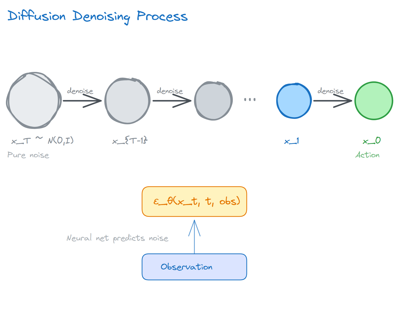
In robotics, the “photograph” is a sequence of actions. During training, you show the model a collection of human demonstrations and let it learn to “denoise”: starting from pure noise, it progressively recovers a reasonable action.

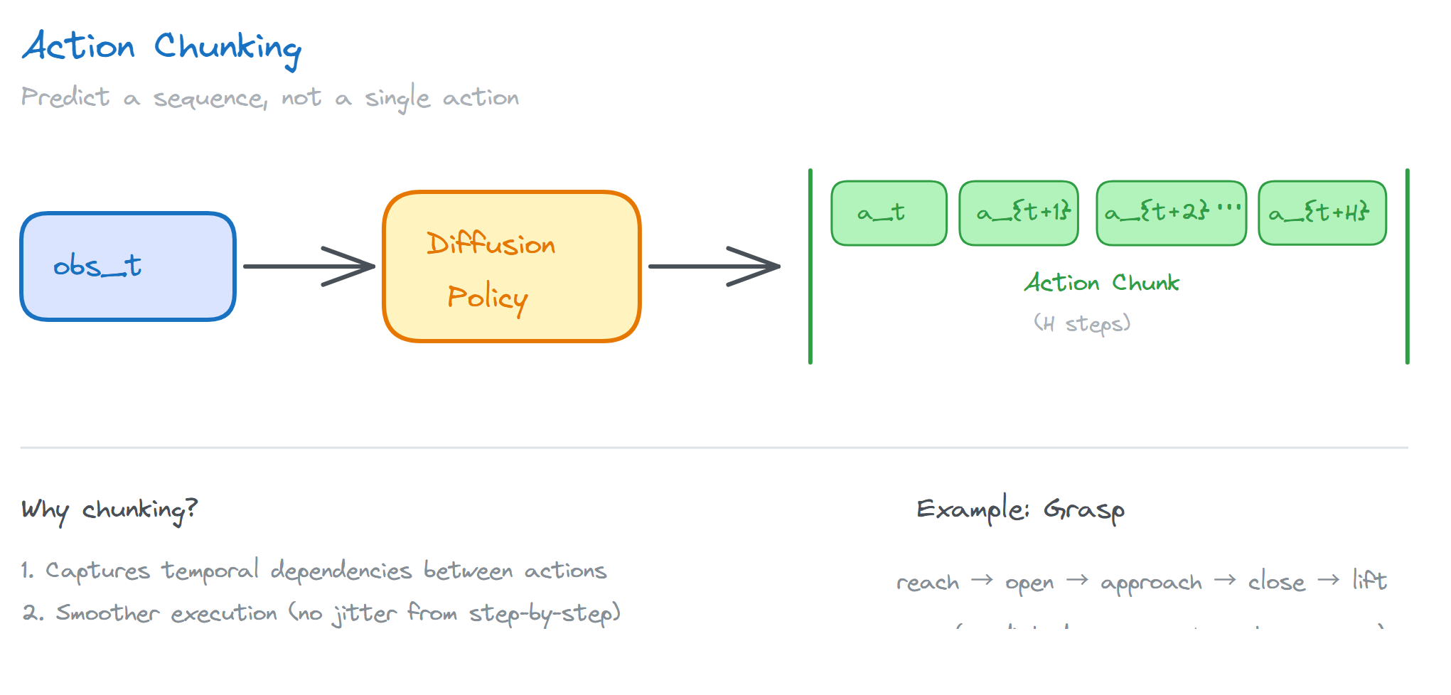
How exactly? Diffusion Policy takes the current observation (images, joint angles, etc.) as input and outputs an action sequence over a future time horizon. The implementation in Chi et al. (2023) features a clever design called action chunking: instead of predicting one action per step, it predicts an entire action sequence and executes it smoothly. This captures temporal dependencies between actions. Think about it: grasping a cup is not a single action but a series of them, reach, open fingers, approach, close, lift. These actions have strong interdependencies. Predicting them one at a time tends to result in jittery motion; predicting them together gives a much smoother result.

Chi et al. (2023) made this idea work well in practice. But it has one fundamental limitation: it can only imitate, not improve. Actions not found in the demonstration data simply won’t appear.

That’s why combining it with RL matters.

But before going further, I want to note something easy to overlook. In the classic framing, the “imitation-only” nature of Diffusion Policy is not a bug but a feature. Precisely because it rigorously learns the data distribution, it guarantees that the generated actions are “reasonable.” If it could freely generate actions outside the data distribution, the “structure” it learned would be meaningless.

The problem is that “reasonable” does not equal “optimal.” Actions in the demonstration data may be reasonable but not the best. Human demonstrators have their own habits, preferences, and even mistakes. Diffusion Policy faithfully learns all of these, including the parts that aren’t so good.

That is the problem RL is here to solve: on the foundation of “reasonable,” find “better.”

Why Combine Them?

What is RL’s strength? Autonomous optimization. Give it a reward signal and it can find better policies through trial and error, without needing human demonstrations.

But RL’s problem is also obvious: exploration is extremely inefficient.

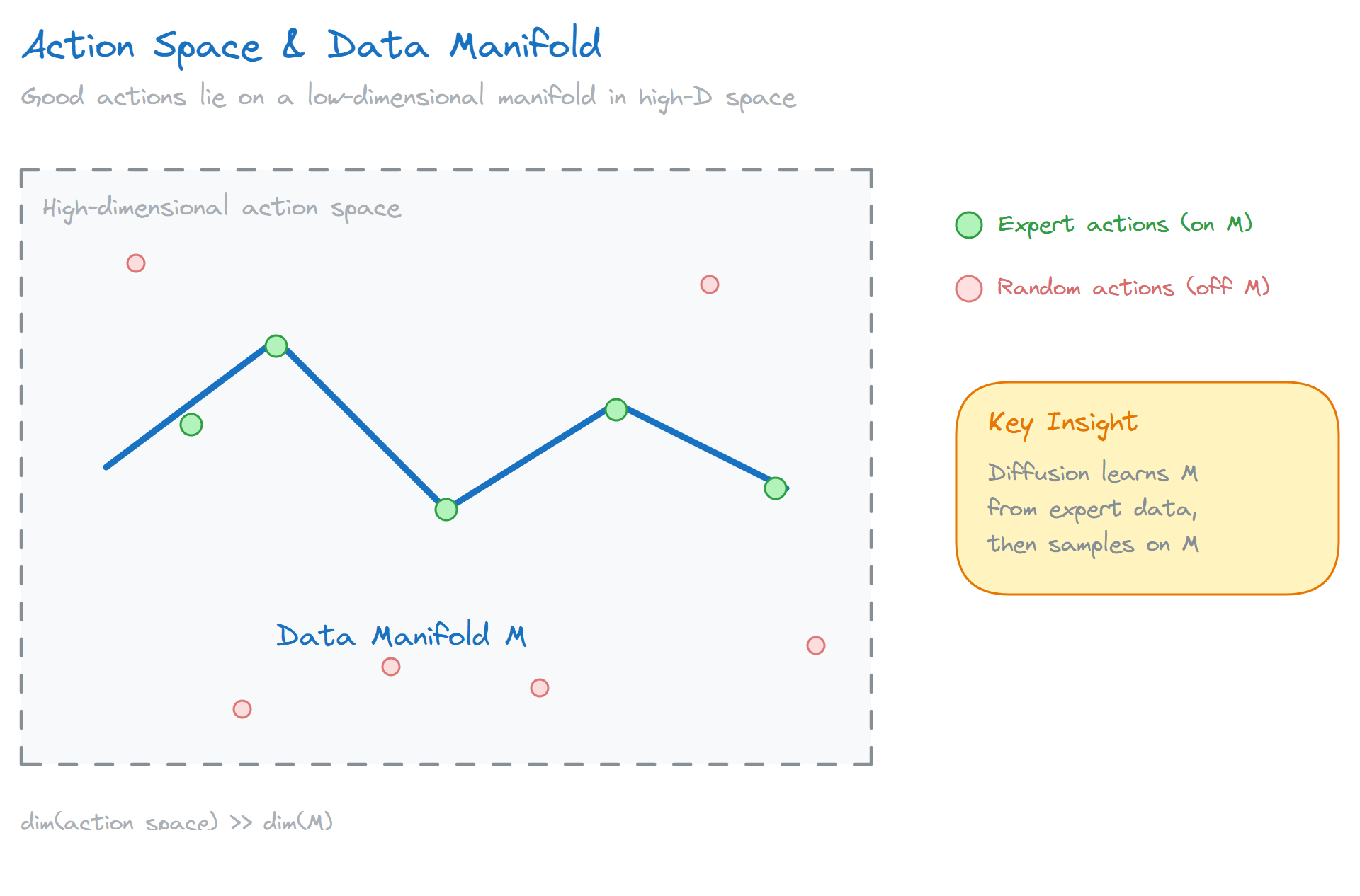
A robot’s action space easily has dozens of dimensions. In such a high-dimensional space, random exploration is essentially searching for a needle in a haystack. The vast majority of attempts are meaningless: either the action is physically unreasonable (joint angles beyond physical limits), or it’s completely mismatched to the current state (the cup is on the left, and the robot reaches right).

How bad is this problem? Let’s do the math. A 7-DOF robotic arm, if each joint has 10 possible velocities, gives $10^7 = 10$ million combinations. With random noise exploration, the probability of finding a good action decreases exponentially with dimensionality. Worse, in high-dimensional spaces, “good actions” are typically concentrated on a low-dimensional manifold. Imagine a 10-million-dimensional space where good actions might occupy only a 100-dimensional thin slice. The probability of random sampling hitting this slice is essentially negligible.

This is why traditional RL has always struggled with robotics. Sample efficiency is too low; real robots simply can’t afford it.

There’s a very practical concern here: every attempt on a real robot has a cost. Time, energy, wear and tear, and safety risks. If an algorithm needs a million attempts to learn a task, it might finish in a few hours in simulation but could take years on a real robot. This isn’t an exaggeration. Many RL algorithms perform well in simulation but completely fail on real robots, and the reason is exactly this: sample efficiency is too low.

So what about combining Diffusion with RL?

Intuitively, this pairing is natural: use Diffusion to learn a distribution over “reasonable actions,” then use RL to find the optimum within that distribution. Diffusion handles “what is reasonable”; RL handles “which is best.”

But might this still be too surface-level?

The reason this combination works may not just be “complementarity.” The generative process in Diffusion itself provides a special mode of exploration, and this point rarely gets discussed.

The Core: What Is Structured Exploration

How does traditional RL explore? Add noise to actions, randomly perturb, and see what happens.

The problem is that this exploration is “unstructured.” You are jumping around in the entire action space, and most jumps land in regions that are “unreasonable.”

Diffusion’s exploration is different.

Diffusion generates actions through an iterative process: starting from pure noise, denoising step by step, until an action emerges. Each denoising step is a small adjustment, not a random jump across the whole space. More crucially, the direction of adjustment is meaningful: it tends to drift toward the region of “reasonable actions.”

The word “manifold” here is literal. Suppose training data (human demonstrations) is concentrated on a low-dimensional submanifold of the action space. The score function that Diffusion learns will point toward the manifold near the manifold. Why? Because the score function points in the direction of fastest increase in probability density. Since the data is on the manifold, probability is low outside the manifold, so the score naturally pulls you toward it. The denoising process moves along this direction, tending to stay close to the manifold.

This is what I mean by “structured exploration”: you are still trying different possibilities, but the range of trying is implicitly constrained to “reasonable” territory. The direction of exploration is no longer random.

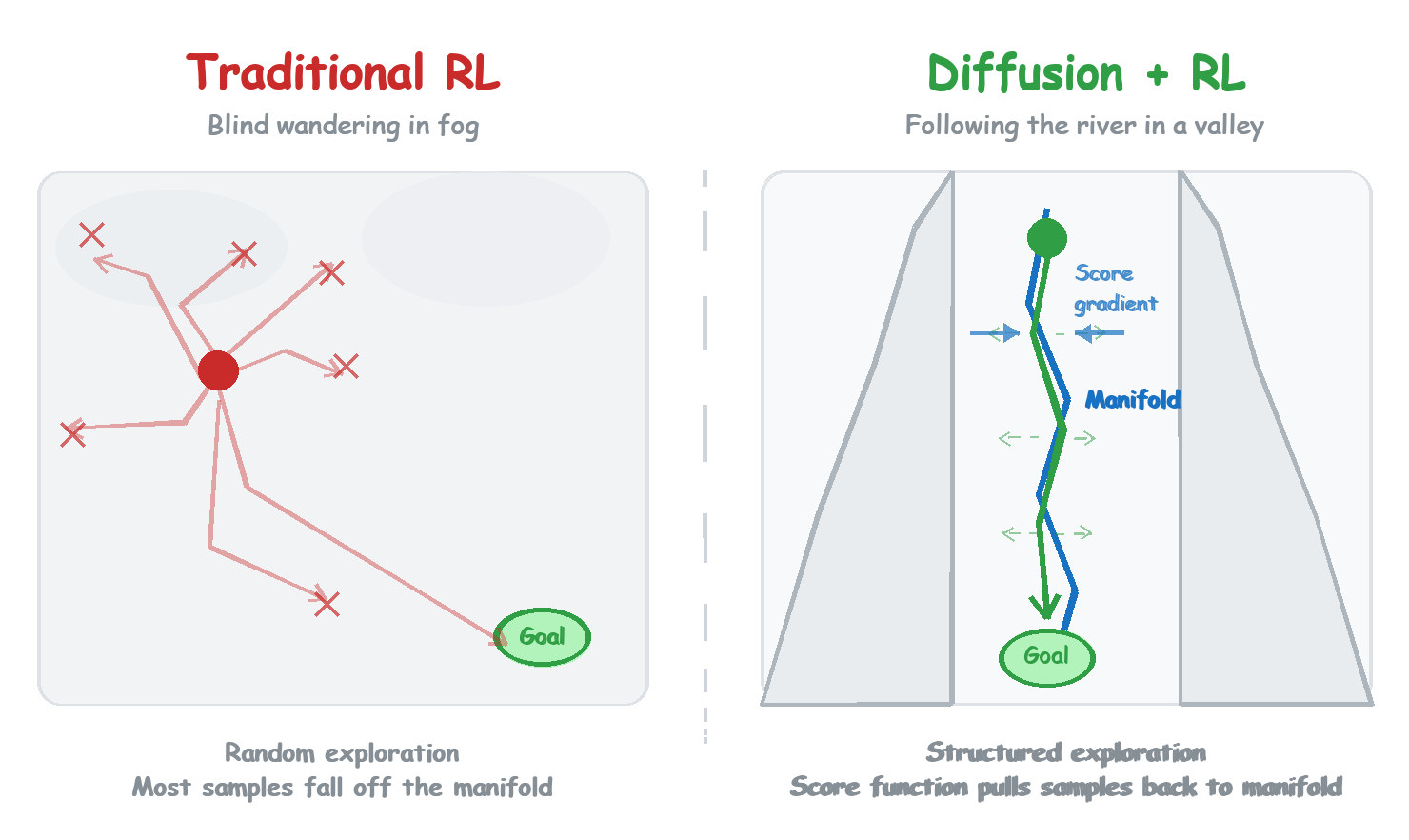
An analogy: traditional RL exploration is like being dropped into a fog-covered mountain range with no map and no landmarks, stumbling around blindly, spending most of the time in dead ends. Diffusion + RL exploration is more like walking along the bottom of a valley. You can still probe left and right, but the steep slopes on either side (the gradient from the score function) exert a constant pull that keeps drawing you back toward a reasonable path. You don’t stray far; each probe lands in territory with a path.

One clarification worth making: structured exploration is not the same as the “constrained exploration” in constrained RL or safe RL. Constrained RL uses explicit constraints; you define a constraint set (e.g., “velocity cannot exceed a certain threshold”) and enforce it during optimization. Structured exploration’s constraint is implicit; it comes from the distribution of the data itself. The manifold Diffusion learns is not something you designed; it “grew” from the demonstration data. Explicit constraints require domain knowledge; implicit constraints are more flexible but harder to debug. The two are complementary, not interchangeable.

Another analogy that might be clearer: a painter at work. No one starts with a blank canvas and random brushstrokes hoping to accidentally produce the Mona Lisa. A painter starts with a sketch, establishing rough composition and proportions, then progressively refines. The sketch is the “structure”; the refinement is the “exploration.” What Diffusion + RL does is similar: first use imitation learning to establish a “sketch” (the distribution of reasonable actions), then use RL to “refine” on top of the sketch (find better actions).

This at least explains why Policy Gradient is surprisingly efficient on Diffusion: exploration is constrained near the manifold, and each gradient update is more meaningful, less likely to be wasted on “unreasonable” directions. Moreover, the iterative structure of Diffusion is naturally suited to progressive optimization. PG’s philosophy is “small steps”; the denoising process is inherently “small adjustments.” The two fit together neatly.

Why Does the Score Function Naturally Point Toward the Manifold?

There is a beautiful mathematical intuition here.

What Diffusion learns is the score function. More precisely, it learns the score of the noise-perturbed distribution at different noise levels, written as $\nabla_{x_t} \log p_t(x_t)$. This has an interesting geometric property: when the data distribution is concentrated on a low-dimensional manifold, the score function near the manifold points toward the manifold itself.

Why? Because the score function points in the direction of fastest increase in probability density. If the data is on the manifold, leaving the manifold means a sharp drop in probability, so the score naturally pulls you back.

Stanczuk et al. (2022, whose original discussion concerns manifold dimension estimation rather than robot control) give a useful result: if the data is concentrated near a low-dimensional manifold, then in the small-noise limit, the score function points in the normal direction toward the manifold.

In plain language: Diffusion doesn’t just know “what the data looks like”; it also knows “what direction is away from the data.” Imagine a sphere: every point on the surface has a direction perpendicular to the surface, pointing outward. What Diffusion learns is these “outward deviation” directions, so it can pull deviated points back.

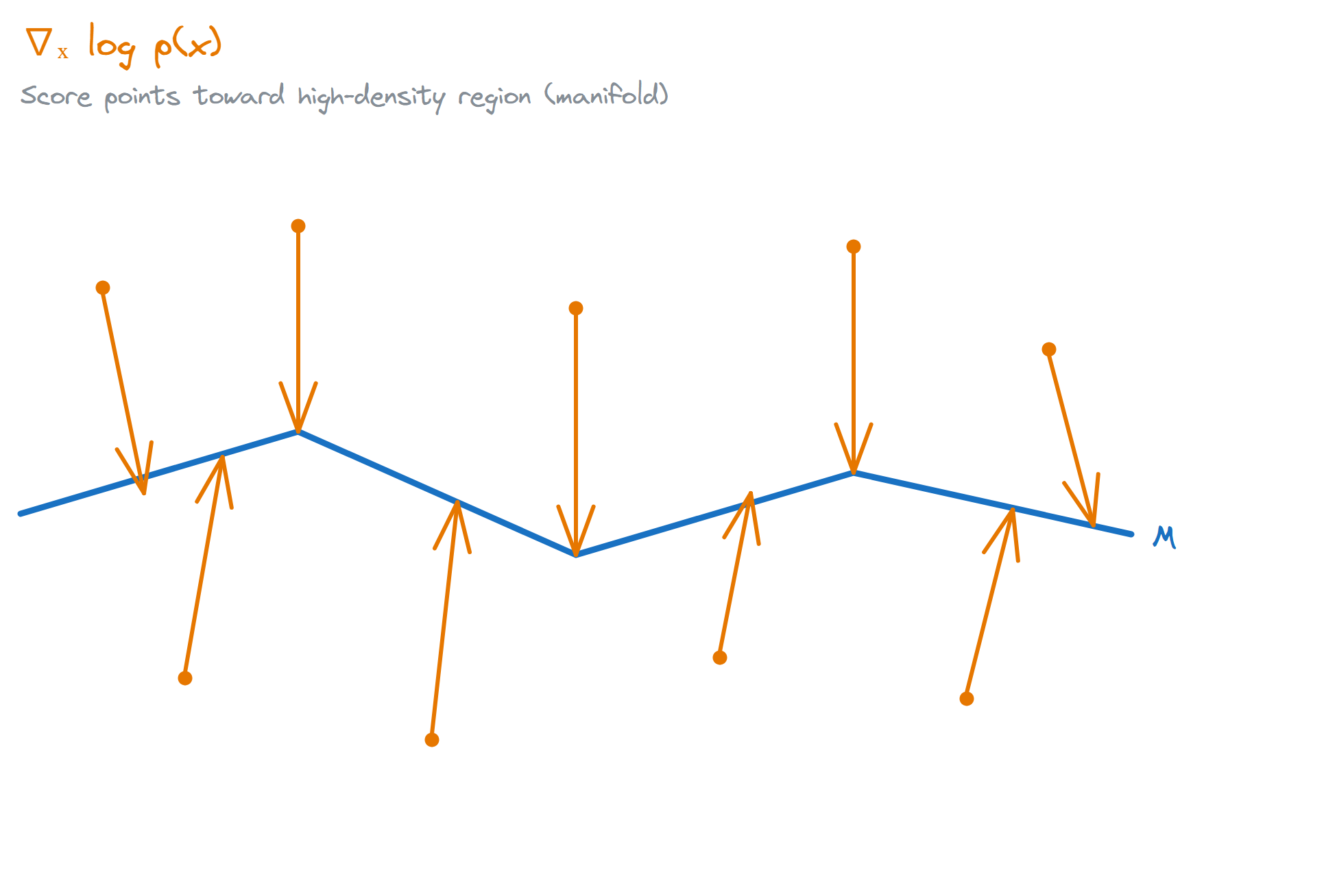
This result sounds dense, but its practical meaning is clear: when the noise level is small, denoising steps tend to pull samples back toward high-probability territory, i.e., closer to the data manifold.

Strictly speaking, this is not performing an exact “projection onto the manifold.” But as a geometric intuition, it is sufficient to explain why the update directions in Diffusion are not arbitrary.

So when we speak of “structured exploration,” the “structure” doesn’t come from nowhere; it is the geometric structure of the data itself. Diffusion, by learning the score function, has implicitly learned the shape of the data manifold.

There is an analogous mathematical perspective here: structured exploration can be approximately understood as KL-Regularized RL. Diffusion Policy provides an extremely powerful prior distribution $\pi_{\text{base}}$. The RL objective is to maximize reward while minimizing the KL divergence between the current policy $\pi$ and $\pi_{\text{base}}$:

\[\max_{\pi}\ \mathbb{E}_{\pi}[R] - \eta \cdot D_{\mathrm{KL}}(\pi \,\|\, \pi_{\text{base}})\]

Traditional RL (such as SAC) uses a Gaussian distribution as the prior, and exploration directions are diffuse. With Diffusion as the prior, the KL divergence constraint acts like an invisible leash, tying exploration to the neighborhood of the data manifold. As I’ll mention later, some recent work has formalized this intuition into a theoretical framework of “entropy maximization on the manifold.”

Staying Close to the Expert Data Manifold

The authors of DPPO use a precise term: on-manifold exploration, or more accurately, exploration around the expert data manifold. Exploration happens near the expert data manifold rather than randomly across the entire action space.

How does traditional RL explore? By adding noise to actions. The problem is that most noise will take you off the manifold, and off-manifold actions are unreasonable to begin with, so this exploration is mostly wasted. Diffusion is different: the denoising process naturally tends to pull samples toward high-probability regions, so exploration is more likely to stay within reasonable bounds. This at least suggests that DPPO’s exploration samples are more tightly distributed along the expert data manifold, rather than simply being more spread out than a Gaussian policy. Whether this is the sole reason for its higher sample efficiency is not yet settled.

There is a compelling experiment in the DPPO paper: the authors visualize the exploration tendencies of different methods in environments like Avoid, finding that the diffusion policy’s exploration coverage stays closer to the expert data manifold, while Gaussian policies tend to scatter further out. This is more telling than simply reporting a benchmark score, because it reveals something more fundamental: the quality of exploration matters more than the quantity.

I think this is one of the most underappreciated perspectives in the whole Diffusion + RL combination. Everyone is discussing how to compute gradients, how to speed things up, but the geometric side of structured exploration may be the key to understanding “why it works.” That said, this is currently more of an experimental observation and geometric intuition than a proven singular mechanism. I find its explanatory power compelling.

What Makes Diffusion Special?

At this point you might ask: BC warm-start already helps RL on its own. How much of this is actually due to Diffusion’s geometric structure?

That’s a good question, and one I’ve thought about for a while.

It’s true that any good initialization helps RL. Pre-train an MLP policy with BC, then fine-tune with PPO, and you’ll do better than starting from scratch. So what’s special about Diffusion?

My understanding is that the distinction lies in the definition of “good.” BC pre-training with an MLP gives you a point estimate, an “average-optimal” action. Diffusion gives you a distribution, a manifold of reasonable actions.

When RL begins exploring, an MLP policy’s exploration adds noise around this point estimate, and the noise direction is arbitrary. A Diffusion policy’s exploration moves along the manifold, in a structured direction.

This is not to say MLP + BC + RL doesn’t work. It does, just with different efficiency. The comparison experiments in the DPPO paper show that, under the same sample budget, Diffusion policy performs noticeably better. Can this gap be fully explained by “better initialization”? Honestly, I haven’t carefully checked whether the BC loss levels are actually comparable in the two cases, so this question remains open for me. Answering it would likely require a more careful ablation: control for the BC loss level, and look only at the efficiency difference in the RL fine-tuning phase.

That said, this is still just one perspective. To rigorously prove that “geometric structure is the key factor,” you’d need more careful ablations: for instance, train a Normalizing Flow on the same data and see if it has similar effects. If so, that suggests the key is “learning the data manifold.” If not, then maybe Diffusion’s iterative denoising process itself is also important.

Current evidence is more indirect. But I lean toward the geometric structure explanation, because it can unify many observations: why exploration is more efficient, why training is more stable, why it’s less sensitive to hyperparameters.

But Maybe I’m Wrong?

Stepping back and viewing this from the outside: I might be over-attributing causality here. My own thinking is still far from settled.

“Structured exploration” is an attractive explanation, but it’s not the only one. Maybe the real reason Diffusion + RL works is something else entirely:

Maybe it’s better initialization. Diffusion pre-training gives a better starting point than MLP, and the subsequent RL is just cashing in on that advantage.

Maybe it’s a more expressive policy class. Diffusion can represent multimodal distributions, which is intrinsically stronger than a Gaussian policy, independent of anything about “manifolds.”

Maybe it’s the smoothness from action chunking. Predicting an entire action sequence is naturally more stable than per-frame prediction; that’s a benefit of temporal modeling, not exclusive to Diffusion.

Maybe it’s training stability from the denoising process. Iterative denoising produces smoother gradients; that’s an optimization-level benefit, separate from “exploration.”

All of these explanations have merit, and they are not mutually exclusive. The true reason is likely a combination of factors rather than a single “structured exploration.”

So why do I still lean toward the geometric structure explanation?

Because it has stronger predictive power. If the key is “learning the data manifold,” then we can predict that any method capable of learning the manifold (Normalizing Flow, VAE, Energy-Based Model) should have similar effects. If the key is only “better initialization,” it becomes hard to cleanly explain the efficiency gap between Diffusion and MLP with that single factor alone.

Of course, this is just my own view. To properly disentangle the contributions of these factors requires more careful ablation experiments. But in the absence of better evidence, I choose to believe the explanation with stronger predictive power.

I think this perspective is undervalued. Most papers emphasize “how to do it” (new algorithm, new loss, benchmark gains), but few systematically discuss “why it works.” If we could more clearly understand the latter, we’d be better equipped to predict “when it will work” and “when it won’t.” To me, that is worth more than reading benchmark rankings.

What This Insight Explains

Having understood structured exploration, many things fall into place. Let’s look at how this insight manifests in specific methods.

DPPO: The Denoising Chain as an MDP

As mentioned earlier, the difficulty was never in the Policy Gradient paradigm itself, but in how you write the policy object. DPPO’s approach is: don’t model the final action directly; optimize each step of the denoising chain. Each step is an analytically tractable Gaussian, so log probability can be computed directly and PPO runs without modification.

Concretely, it treats the entire denoising chain as an MDP: each denoising step is an “action,” and the entire chain is an episode. The denoising process is inherently progressive; each step can be independently evaluated and optimized. This doesn’t work around Diffusion’s intractable likelihood; it exploits the step-by-step structure of the denoising process.

Technically, DPPO uses a two-level MDP design:

The outer MDP is the robot’s interaction with the environment. The state is the observation, the action is the full action sequence, and the reward is whether the task succeeded.

In the inner MDP (the denoising process), the state is the action at the current noise level, and the action is a single denoising step. The reward, however, is where it gets tricky: the denoising process itself has no reward; reward only appears at the end of the outer MDP.

The solution is index flattening.

Flatten the two-level MDP into one long episode. If the outer level has $T$ steps and the inner denoising has $K$ steps, the whole episode is $T \times K$ steps. Then use standard GAE (Generalized Advantage Estimation) to estimate the advantage at each step.

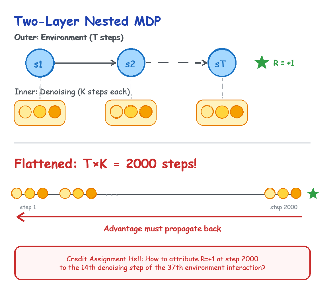
What is GAE? Simply put, it’s a method for “assigning credit.” You received a reward at the end, but that reward was the result of many prior actions. GAE estimates how much each step contributed to the final reward. It uses a decay factor $\lambda$ to balance “short-term influence” and “long-term influence”: steps closer to the reward get more credit, those farther away get less, but are not ignored entirely.

\[\hat{A}_t = \sum_{l=0}^{\infty} (\gamma \lambda)^l \delta_{t+l}, \qquad \delta_t = r_t + \gamma V(s_{t+1}) - V(s_t)\]

(Strictly speaking, DPPO’s implementation is more complex: it uses environment-step GAE combined with a denoising discount, rather than running standard GAE on every denoising step. But the core idea is the same: pass the reward signal from the outer level down to the inner denoising process.)

The elegance of this design is that the reward from the outer MDP (task success) can be propagated to each denoising step via GAE. Even though early denoising steps are far from the final reward, GAE allocates credit based on value estimates from subsequent steps.

But this elegant design comes with significant engineering cost.

Suppose the outer robot-environment interaction takes $T=100$ steps to receive a sparse reward (picking up the cup), and the inner Diffusion denoising takes $K=20$ steps. After flattening, PPO faces a super-long episode of 2,000 steps. What RL fears most is the credit assignment problem: the robot receives a reward of $+1$ at step 2,000; how should GAE precisely distribute that credit back to the 14th denoising step during the 37th environment interaction? Such extreme episode lengths lead to very high variance in advantage estimates.

DPPO’s approach is to handle the decay for environment rewards and denoising steps separately. The paper’s description of this part is not particularly detailed, but based on the method design, this separation seems to be the key that makes credit assignment tractable. This may also be why DPPO is somewhat sensitive to hyperparameters; at least from the ablation experiments in the paper, the choice of discount factor has a noticeable effect on performance.

That said, this path works for a crucial reason: in DPPO’s parameterization, each denoising step corresponds to an analytically tractable Gaussian likelihood, meaning log probability can be computed directly without needing to handle the intractable marginal likelihood of the full Diffusion model. This is why PPO can be applied directly.

Why is the likelihood of original Diffusion intractable? Because given an action $a$, its likelihood requires integrating over all possible denoising paths:

\[p(a) = \int p(a \mid x_{1:T}) p(x_{1:T}) \, dx_{1:T}\]

This integral has no closed-form solution. But DPPO sidesteps the problem: it doesn’t need the likelihood of the entire trajectory, only the likelihood of each individual denoising step. In this step-by-step parameterization, each step has an analytically tractable Gaussian likelihood; log probability can be computed directly. The importance sampling ratio that PPO requires becomes the product of per-step ratios under the flattened MDP, fully computable:

\[\prod_{k=1}^{K} \frac{p_\theta(x_{k-1} \mid x_k, s)}{p_{\theta_{\mathrm{old}}}(x_{k-1} \mid x_k, s)}\]

Note that what’s being computed here is the joint probability ratio of the entire denoising chain, not the marginal likelihood ratio of the final action.

So sometimes the way to circumvent a hard problem is to change perspective until the problem becomes irrelevant. DPPO didn’t solve the intractable likelihood problem in Diffusion; it simply discovered that if you treat the denoising process as an MDP, the problem doesn’t need to be solved.

From the structured exploration perspective, DPPO’s contribution is not a new algorithm per se, but a shift in perspective: reinterpreting Diffusion’s generation process as an MDP that can be optimized with RL. This shift allows you to fine-tune the policy with PPO while preserving the manifold structure Diffusion learned.

Offline RL: Diffusion as a Constraint

The other technical direction is Offline RL, with Diffusion-QL as the representative work.

The core problem in Offline RL is distribution shift: Q-learning pushes the policy toward high-Q actions, but if those actions weren’t seen in the training data, Q-value estimates are unreliable. Traditional methods use various regularization techniques to prevent the policy from straying too far, with mixed results.

The key in Diffusion-QL is that it directly incorporates action-value maximization into the training objective of the diffusion policy, rather than simply adding a Q-gradient at sampling time:

\[\mathcal{L}_{\mathrm{Diffusion\text{-}QL}} = \mathcal{L}_{\mathrm{diffusion}} - \alpha \cdot \mathbb{E}_{x_0 \sim \pi_\theta(\cdot \mid s)}\left[Q_\phi(s, x_0)\right]\]

The paper’s framing is to fold “maximizing action-values” directly into the training loss of the conditional diffusion model. This way, the policy both retains its fit to the behavior policy and is nudged toward actions with higher Q values.

Put differently, Diffusion-QL couples behavior cloning and policy improvement into a single objective, rather than applying additional guidance during sampling. This is also structured exploration in action: Diffusion first constrains the policy near the behavioral data, then RL pushes it toward more optimal directions within that range. The manifold constraint is encoded directly into the policy, rather than applied as a temporary operation at sampling time.

After Diffusion-QL, EDP (Efficient Diffusion Policy) addressed a practical bottleneck: training was too slow. The numbers in the paper’s abstract are striking. On the D4RL locomotion benchmark, relative to the official Diffusion-QL implementation, diffusion policy training time was reduced from 5 days to 5 hours (the exact numbers depend on the task and hardware). The core idea is to approximate actions from corrupted actions during training rather than running the full diffusion chain each time. This shows that this line of work is not only conceptually valid but also engineering-mature.

Worth mentioning here are two earlier works: Janner et al. (2022)’s Diffuser and Ajay et al. (2023)’s Decision Diffuser. These were pioneering applications of Diffusion to sequential decision-making, using Diffusion to model entire trajectories rather than just actions. Diffusion-QL and EDP can be seen as extensions of that line in the direction of policy learning.

Inference-Time Guidance: The Frozen-Weights Route

The methods discussed so far all combine Diffusion and RL at training time. Here I’ll take a brief detour. It is not the main line, but it helps illustrate that “structure-preserving, then navigating” doesn’t have to happen during training. It can happen at inference time.

The core idea is: why do we have to use RL to fine-tune the model’s weights at all? Since Diffusion has already learned the structure of the data distribution (the score function), we can freeze the Diffusion weights entirely and train only an additional Q-function.

During generation (denoising), we add the gradient of the Q-value as extra guidance, in the style of classifier-free guidance, layered on top of the denoising direction. Schematically:

\[x_{t-1} \approx \mu_\theta(x_t, t) + \alpha \nabla_{x_t} Q_\phi(x_t)\]

The intuition:

Each step = follow the learned score field + move toward higher reward ($\alpha \nabla Q(x)$)

One advantage of this approach is that the base Diffusion model’s weights are untouched, so it is less likely to directly overwrite the original distribution the way training-time fine-tuning can. More precisely, it navigates by referencing the learned structure. Diffusion draws the track; Q-gradient presses the accelerator within that track.

Of course, this approach has its own issues: Q-function estimation needs to be sufficiently accurate, and the computational overhead during inference increases. But for settings where you are especially concerned about mode collapse, or where you don’t want to retrain a large model, this is a viable option worth considering. It shifts “improvement” from training time to inference time, accepting slower inference in exchange for preserving the already-learned structure.

Flow Matching: Faster Structured Generation

Physical Intelligence’s $\pi_0$ series uses Flow Matching rather than Diffusion. But the underlying idea is the same.

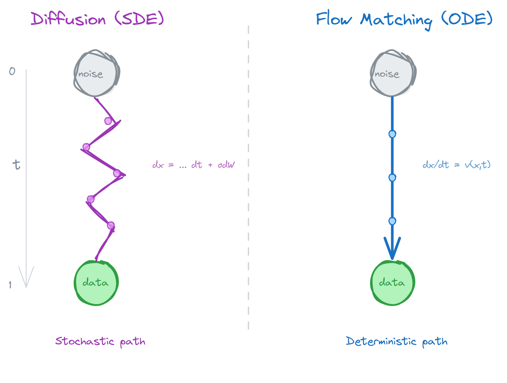
The difference between Flow Matching and Diffusion can be roughly understood as a different path shape: Diffusion corresponds to a stochastic denoising process; Flow Matching learns a velocity field that continuously pushes noise toward the data distribution.

An analogy: Diffusion is like navigating a maze by random walk, with noise at each step but a general drift toward the exit. Flow Matching is more like having a map that tells you the shortest path from your current position to the exit. Both eventually reach the exit, but Flow Matching’s path is more direct and more efficient.

Mathematically, Flow Matching learns a velocity field $v(x, t)$ satisfying:

\[\frac{dx}{dt} = v(x, t)\]

Integrating from $t=0$ (noise) to $t=1$ (data) traces a continuous generation trajectory. The key difference is that Diffusion’s path is stochastic (SDE), while Flow Matching’s is deterministic (ODE). Deterministic paths mean fewer sampling steps are needed to obtain high-quality results.

This speed advantage is especially important in robot control. In systems like $\pi_0$, the authors use approximately 10 Flow Matching steps to predict an action chunk, in principle making high-frequency control feasible. But the model being able to output action chunks quickly is one thing; real-time execution at the system level is another. Black et al. (2025) subsequently proposed the RTC (Real-Time Chunking) algorithm specifically to address the real-time execution of action chunking flow policies.

But Flow Matching has its own tradeoffs. Thinking of it as “a more direct, deterministic generation path” is fine, but don’t read this as proving that the optimal path from noise to data is always a straight line. More accurately, it selects a class of path parameterizations that are easier to train and easier to numerically integrate. For complex multimodal distributions (e.g., “left-hand grasp” and “right-hand grasp” as two modes), these more direct paths may not always be ideal and could introduce a tradeoff between expressiveness and efficiency.

$\pi_{0.5}$: From Manipulation to Generalization

$\pi_{0.5}$ is more of an extension of this direction toward open-world generalization. The paper emphasizes heterogeneous co-training and hybrid multimodal examples: training on data from different sources and modalities together, so the model is not only capable of specific tasks but possesses cross-scenario generalization.

$\pi^{*}_{0.6}$ / RECAP: Continuing to Improve on Existing Structure

The RECAP method in $\pi^{*}_{0.6}$ centers on advantage conditioning. The workflow is: first pre-train a VLA with offline RL, then collect autonomous rollouts in a real environment, add expert corrective interventions as needed, train a value function to estimate advantages, and finally use advantage-conditioned policy extraction to update. The technical details differ from DPPO, but it addresses the same problem: how to keep improving a policy while preserving its existing structure.

The benefit of this approach is that it rewrites “directly online-optimizing a large VLA” into a more controllable advantage-conditioned update pipeline. For real robots, this rewrite matters, because it makes it easier to incorporate demonstrations, rollouts, and interventions into the same training loop.

---

Looking back at this collection of methods, they share a common thread: how to make a policy better while preserving some form of “structure.”

Method	Structure Preserved	Mode of Improvement
DPPO	Iterative structure of the denoising process	PPO on flattened MDP
Diffusion-QL	Manifold constraint encoded in training objective	Q-value maximization
Inference-time guidance	All model weights frozen	Q-gradient at inference
Flow Matching	Deterministic generation path	Faster action chunks
RECAP	Semantic prior from large model	Advantage conditioning

Different forms, but the same core idea: don’t start from scratch. Improve on top of existing structure.

What This Perspective Can Help You Do

We’ve spent a lot of space on “why it works.” But understanding mechanisms is not the goal; the goal is to guide practice. If the structured exploration perspective is correct, it should help us make better method choices, not just look for whichever benchmark score is highest.

Considerations for Method Selection

If you’re building a project with a real robot right now, which route should you take?

I think DPPO is the more practical choice. Three reasons:

First, the workflow is clear. Collect demonstrations, train Diffusion Policy, then fine-tune with RL. Each step has a clear objective and verifiable results. You don’t want a black box; you want a system you can debug incrementally.

Second, it’s real-robot-friendly. No need to train Diffusion online (that’s too slow); you only need to fine-tune an existing policy. Computational overhead is manageable, and sample efficiency is high.

Third, the two-level MDP design is elegant. It naturally unifies Diffusion’s generation process with RL’s optimization; not a forced marriage.

Of course, this is based on the papers I’ve read and my understanding of real-robot scenarios. If your setting is different (pure simulation, training time doesn’t matter), the conclusion may differ.

The Diffusion-QL route is theoretically elegant: use Diffusion to define “what is reasonable,” use Q-learning to find the optimum within that space. But I haven’t seen many successful cases on real robots yet, possibly due to issues inherent to Offline RL (inaccurate Q-value estimation), or because Diffusion’s sampling speed limits real-time control.

Flow Matching surprised me with its speed. If your task requires high-frequency control (e.g., fine manipulation), this route deserves serious consideration. As discussed earlier, there may be a tradeoff on multimodal distributions, but for robot control specifically, the speed advantage currently looks more significant.

The Reward Problem

There’s still one unavoidable issue: reward. Use RL and you have to tell the robot what “good” means. Easy in simulation; painful in the real world.

My current sense is that, given a good imitation initialization, a clear success signal, and a task structure close to the DPPO paper’s settings (e.g., manipulation tasks like Lift and Can), sparse reward (success +1, failure 0) may already be sufficient. Worth noting though: in the DPPO paper’s own task list, locomotion tasks (Hopper, HalfCheetah) still use dense reward, so the scope of this conclusion is narrower than intuition suggests. The structure narrows the exploration range, but how narrow depends on the specific task and initialization quality.

There’s an interesting tradeoff here: the sparser the reward, the higher the demand on initialization; the denser the reward, the heavier the reward engineering burden.

This makes me think of a more general question: the relationship between reward design and prior knowledge. The traditional RL approach is to “encode all prior knowledge in the reward”: whatever you want the robot to do, design a reward to guide it there. This is hard, because the reward needs to precisely reflect your intent, and human intent is often vague and difficult to quantify.

Diffusion + RL suggests an alternative: encode prior knowledge in data. Human demonstrations carry a wealth of implicit priors: what constitutes a reasonable action, what makes a trajectory natural, what behaviors are safe. Diffusion learns all of these, and RL only needs to fine-tune on top. The reward engineering burden is genuinely lighter.

The Dark Side of the Manifold: When Structure Bites Back

After all this praise for structured exploration, it’s time for a reality check.

Structure is a double-edged sword. It makes exploration more efficient, but it also draws an invisible boundary around what exploration can reach.

Data Bias Gets Baked Into the Manifold

If the training data itself is biased, the manifold Diffusion learns will be biased. Exploring on a biased manifold, you will never reach the good solutions that lie outside it.

An example: if all demonstration data shows right-hand grasping, Diffusion learns a “right-hand grasping” manifold. Even if left-hand grasping is better in certain situations, RL will have great difficulty discovering that, because exploration is constrained to the right-hand grasping territory.

This is not a problem specific to Diffusion + RL; it affects all imitation-learning-based methods. But structured exploration makes the problem more insidious: you think you’re exploring, but you’re actually circling within a limited space.

RL Can Destroy the Diversity That Diffusion Built

There’s an even more insidious problem: RL may erase the multimodal structure that Diffusion worked hard to capture.

One of Diffusion Policy’s greatest selling points is multimodality. Facing a cup, expert demonstrations might show 5 different grasps, and Diffusion faithfully preserves all 5 peaks. But RL is an extremely greedy optimizer. If in simulation RL discovers that “right hand, top-down grasp” gives a reward of 1.01 while the other 4 approaches all give 1.00, RL’s gradient update will mercilessly concentrate all probability mass on that 0.01 advantage.

The result? After RL fine-tuning, the Diffusion model may degrade into a policy that only outputs a single action. It scores higher on the current environment reward, but loses robustness against physical disturbances. If the right hand is blocked, it can no longer switch to the left, because the left-hand manifold has been erased by RL.

This is called mode collapse. At its core, it’s the same problem as data bias viewed from the other side: data bias means the manifold was incomplete to begin with; mode collapse means RL trimmed down a manifold that was originally complete. What they share: the structure is shrinking, not expanding.

Is There a Way Forward?

How do you solve these problems? Honestly, there are no great answers yet.

To combat mode collapse, a common approach is to add a KL divergence constraint to the RL loss:

\[\mathcal{L}_{\mathrm{total}} = \mathcal{L}_{\mathrm{RL}} + \beta \cdot D_{\mathrm{KL}}(\pi_\theta \,\|\, \pi_{\mathrm{base}})\]

This prevents the fine-tuned policy from straying too far from the original Diffusion. Another approach adds an entropy penalty to encourage the policy to maintain diversity. Barceló et al. (2024) proposed Hierarchical Reward Fine-tuning, using dynamic hierarchical training to avoid mode collapse. But these methods tend to reduce the performance ceiling. Maintaining diversity and maximizing reward are in fundamental tension.

As for data bias, I can think of a few possible directions, none of which qualify as mature answers yet.

$\epsilon$-greedy off-manifold exploration: most of the time explore on the manifold, but with small probability apply a large random perturbation to forcibly jump off the manifold and see what’s out there. Crude, but sometimes crude methods actually work.

Multi-manifold ensemble: train multiple Diffusion models, each on a different data subset, covering different modes. At inference time, use a meta-policy to select which model to use.

Active data collection: if you notice the current model only grasps with the right hand, go specifically collect left-hand grasping demonstrations, then retrain or fine-tune Diffusion. This requires a human in the loop, but may be the most reliable approach.

All of these have their own issues. But at minimum we should be aware that the problems exist, rather than assuming structured exploration can solve everything.

Structure vs. Randomness: A Deeper Distinction

Earlier I mentioned that structured exploration can be understood as KL-Regularized RL. This analogy can be pushed further.

What is RL fundamentally doing? It is reweighting the policy distribution: increasing the probability of good actions, decreasing that of bad ones. BC provides an initial distribution; RL repeatedly reweights on top of it, progressively shifting probability mass toward high-reward regions.

More concretely: under KL constraint, the optimal update policy has a clean closed-form solution:

\[\pi^{*}(a \mid s) \propto \pi_{\text{base}}(a \mid s) \cdot \exp\!\left(\frac{Q(s, a)}{\eta}\right)\]

where $Q(s,a)$ is the action-value function and $\eta$ is the temperature parameter. This means every RL update is fundamentally a reweighting of the current distribution. Good trajectories gain weight; bad trajectories lose it.

The critical question is: in which space does the reweighting occur? Traditional RL models the policy with a Gaussian distribution; reweighting happens across the entire action space, but most probability mass is outside the manifold, making adjustments to those regions wasteful. The distribution that Diffusion learns is already concentrated on the data manifold; reweighting occurs within the manifold. This is the efficiency source of structured exploration: every reweighting is more meaningful, not just fewer in number.

There is a recent paper (De Santi et al., 2025) that formalizes this intuition: it writes the exploration problem as entropy maximization on the data manifold:

\[\max_{\pi} H(\pi) \quad \text{s.t.} \quad \operatorname{supp}(\pi) \subseteq \mathcal{M}_{\mathrm{data}}\]

where $\mathcal{M}_{\mathrm{data}}$ is the data manifold and $H(\pi)$ is the policy entropy. Their idea is that a pre-trained Diffusion model implicitly defines an approximate data manifold, and exploration can be written as entropy maximization over this constrained region. This paper’s experiments are in text-to-image settings rather than robot fine-tuning, but it provides a formal language: if a generative model has already given you a “reasonable region,” exploration is about spreading out as much as possible within that region, rather than searching randomly across the whole space.

From this perspective, mode collapse is fundamentally entropy decreasing as the manifold collapses. RL’s greedy optimization compresses an originally spread-out distribution into a sharp spike.

Structure Determines Boundaries

The traditional machine learning paradigm treats “exploration” and “exploitation” as two separate things that must be balanced manually. But Diffusion’s structure hints at another possibility: exploration itself can be structured, and structure is itself a form of prior.

This leads me to a more general question: how do we inject prior knowledge into AI systems?

Traditional approaches design rewards, losses, and architectures. These are “hard-coded” priors that require domain expertise. But Diffusion + RL demonstrates another possibility: using data to “soft-code” priors. Human demonstrations carry a wealth of implicit priors: what constitutes a reasonable action, what makes a trajectory natural, what behaviors are safe. Diffusion learns all of these; RL only needs to fine-tune on top.

But this paradigm also has its ceiling. If structure determines exploration efficiency, then who determines the boundary of the structure?

Data determines structure, but data is collected by humans. Human biases, human blind spots, the upper limit of human imagination: all of these get baked into the structure. The manifold Diffusion learns is fundamentally the capability boundary of the human demonstrators. RL can find more optimal solutions within this boundary, but it cannot cross it.

Perhaps this is the true ceiling of the Diffusion + RL paradigm: not an algorithm problem, not a compute problem, but a data problem. Demonstration data doesn’t just give you a starting point; it quietly draws the boundaries of exploration.

Structure in, structure out.

---

Written on 2026-03-12

References

1. Chi, C., Xu, Z., Feng, S., Cousineau, E., Du, Y., Burchfiel, B., Tedrake, R., & Song, S. (2023). Diffusion Policy: Visuomotor Policy Learning via Action Diffusion. arXiv:2303.04137

2. Ren, A. Z., Lidard, J., Ankile, L. L., Simeonov, A., Agrawal, P., Majumdar, A., Burchfiel, B., Dai, H., & Simchowitz, M. (2024). Diffusion Policy Policy Optimization. arXiv:2409.00588

3. Wang, Z., Hunt, J. J., & Zhou, M. (2022). Diffusion Policies as an Expressive Policy Class for Offline Reinforcement Learning. arXiv:2208.06193

4. Kang, B., Ma, X., Du, C., Pang, T., & Yan, S. (2023). Efficient Diffusion Policies for Offline Reinforcement Learning. arXiv:2305.20081

5. Stanczuk, J., Batzolis, G., Deveney, T., & Schönlieb, C.-B. (2022). Your diffusion model secretly knows the dimension of the data manifold. arXiv:2212.12611

6. Black, K., Brown, N., Driess, D., et al. (2024). π0: A Vision-Language-Action Flow Model for General Robot Control. arXiv:2410.24164

7. Physical Intelligence, Black, K., Brown, N., et al. (2025). π0.5: a Vision-Language-Action Model with Open-World Generalization. arXiv:2504.16054

8. Physical Intelligence, Amin, A., et al. (2025). π*0.6: a VLA That Learns From Experience. arXiv:2511.14759

9. Black, K., Galliker, M. Y., & Levine, S. (2025). Real-Time Execution of Action Chunking Flow Policies. arXiv:2506.07339

10. Lipman, Y., Chen, R. T. Q., Ben-Hamu, H., Nickel, M., & Le, M. (2022). Flow Matching for Generative Modeling. arXiv:2210.02747

11. De Santi, R., Vlastelica, M., Hsieh, Y.-P., Shen, Z., He, N., & Krause, A. (2025). Provable Maximum Entropy Manifold Exploration via Diffusion Models. arXiv:2506.15385

12. Barceló, R., Alcázar, C., & Tobar, F. (2024). Avoiding mode collapse in diffusion models fine-tuned with reinforcement learning. arXiv:2410.08315

13. Janner, M., Du, Y., Tenenbaum, J. B., & Levine, S. (2022). Planning with Diffusion for Flexible Behavior Synthesis. arXiv:2205.09991

14. Ajay, A., Du, Y., Gupta, A., Tenenbaum, J., Jaakkola, T., & Agrawal, P. (2023). Is Conditional Generative Modeling all you need for Decision-Making? arXiv:2211.15657

Further Reading

Finzi et al. (2026) proposed the Epiplexity framework (arXiv:2601.03220), attempting to answer a foundational question: for a computationally bounded observer, what kind of information is actually “useful”? Their core distinction is that not all “uncertainty” is alike. Epiplexity (extractable structural complexity) refers to the part you don’t yet know the answer to but could infer from data given enough compute; time-bounded entropy, by contrast, is noise that remains unpredictable no matter how much you compute. This distinction resonates deeply with the intuition behind structured exploration: information on the manifold Diffusion learns is high-epiplexity (complex but structured and learnable), while off-manifold territory is more like noise for a computationally bounded agent. The efficiency advantage of structured exploration, translated into this language, is about concentrating samples in regions where structure can be extracted, rather than wasting them in high-entropy, low-epiplexity random space.